# install.packages("remotes")
remotes::install_github("giocomai/castarter")Extracting textual contents from the Kremlin’s website with castarter
tutorials
russia
A first introduction to extracting textual contents for further analysis
Tip
If you are not interested in understanding the details of how this works, you may just skip directly to the processed dataset, ready for download.
Work-in-progress
This page is still a work-in-progress. It is shared in the spirit of keeping the research process as open as possible, but it still a draft document, possibly an early draft: incomplete, unedited, and possibily inaccurate. Datasets included may likewise not be fully verified.
 Context
This is a tutorial demonstrating how to extract textual contents with metadata from the Kremlin’s website using castarter, a package for the R programming language.
As this is an introductory post, all steps and functions are explained in detail.
Step 1: Install castarter
This tutorial assumes some familiarity with the R programming language. At the most basic, you should have installed R and an IDE such as Rstudio, start a new project, and then you can just copy/paste and run commands in a scripts and things should work. Once your setup is in place, make sure you install castarter.
Step 2: Think of file and folder locations
Everyone organises stuff on their computer in their own way. But when getting ready to retrieve hundreds of thousands of pages, some consideration should be given to organising file in a consistent manner.
With castarter, by default, everything is stored in the current working directory, but a common pattern for castarter users will be to keep the file with their R script in a location, often a synced folder, and then to have all the html pages stored for text mining in a non-synced folder. This is because it is common to get hundreds of thousands of pages even for relatively small projects, and storing very large number of small files slows down sync clients for the likes of Dropbox, Google Drive, and Nextcloud. If you rely on git-based approaches, you will need to add the data folders to your .gitignore.
The following setup will store all files in a subfolder of your R installation folder; set it to whatever works for you in the base_folder parameter.
The following code sets a few option for the current session. You will typically want to have something like this at the beginning of each castarter script.
This sets:
- a
base_folder- everything will happen starting from there - a
project- which will generate a folder within thebase_folder. In this case, I’ll set this to “Russian institutions”, as I plan to store here a number of textual datasets from relevant websites, including the website of the Russian president, the Ministry of defence, and the Ministry of Foreign affairs. - a
website- you are free to call it as suits you best, but I have grown accustomed to use the bare domain, an underscore, and then the main language, so in this case it will bekremlin.ru_en(so that it’s easy to differentiate from the Russian language version, which would bekremlin.ru_ru). This is however just a convention, and anything will work.
library("castarter")

cas_set_options(
  base_folder = fs::path(fs::path_home_r(),
                         "R",
                         "castarter_tadadit"),
  project = "Russian institutions",
  website = "kremlin.ru_en"
)
By default, castarter stores information about the links and downloaded files in a local database, so that it will always be possible to determine when a given page was downloaded, or where a given link comes from. By default, this is stored in a SQLite database in the website folder.
Each time a file is downloaded or processed, by default relevant information is stored in the local database for reference.
Step 3: Get the urls of index pages
Conceptually, castarter is based on the idea common to many text mining projects that there are really two types of pages:
- index pages: they are, e.g, lists to posts or articles, the kind of pages you ofen see if you click on “See all news”. Sitemap files can also be understood as index pages in this context. The key part is that these pages are mostly dynamic, and we mostly care about them because they include links to the pages we are actually interested in.
- content pages: these are the pages we mostly actually care about. They have unique urls, and their content is mostly expected to remain unchanged after publication.
In the case of the Kremlin’s website, we can quickly figure out that index pages have these urls:
- http://en.kremlin.ru/events/president/news/page/1 (the latest posts published)
- http://en.kremlin.ru/events/president/news/page/2 (previous posts)
- http://en.kremlin.ru/events/president/news/page/3 (etc.)
- …
Incidentally, I’ll also point out that there’s a version of the website aimed to the visually impaired:
http://en.special.kremlin.ru/events/president/news
We will stick to the standard version in this tutorial to keep things interesting, but it is worth remembering that websites may have alternative versions, e.g. a mobile-focused version, that have less clutter and may be easier to parse. For example, from that version of the website it is easier to see how many index pages there are.
At the time of writing, there are 1350 index pages for the news section of the website. This is how those urls look:
cas_build_urls(url = "http://en.kremlin.ru/events/president/news/page/",
               start_page = 1,
               end_page = 1350)
# A tibble: 1,350 × 3
id url index_group
<dbl> <chr> <chr>
1 1 http://en.kremlin.ru/events/president/news/page/1 index
2 2 http://en.kremlin.ru/events/president/news/page/2 index
3 3 http://en.kremlin.ru/events/president/news/page/3 index
4 4 http://en.kremlin.ru/events/president/news/page/4 index
5 5 http://en.kremlin.ru/events/president/news/page/5 index
6 6 http://en.kremlin.ru/events/president/news/page/6 index
7 7 http://en.kremlin.ru/events/president/news/page/7 index
8 8 http://en.kremlin.ru/events/president/news/page/8 index
9 9 http://en.kremlin.ru/events/president/news/page/9 index
10 10 http://en.kremlin.ru/events/president/news/page/10 index
# ℹ 1,340 more rowsOn many websites, the main “news” section will include links to all relevant articles. In our case, we see that the Kremlin has also a few more sections:
- News
- Speeches and transcripts
- Presidential Executive Office
- State Council
- Security Council
- Commissions and Councils
As it turns out, “Speeches and transcripts” seem to be mostly included in the news feed, but e.g. items from the “Commissions and councils” are not. Less we miss some materials, we may want to get all of these. Or, depending on the research we’re working on, we may be interested only in “Speeches and transcripts”. Either way, to distinguish among different feeds and facilitate future steps, including possibly automatic updating of the procedure, castarter includes an index_group parameter.
So we can build urls separated by index_group, and store them in our local database.
cas_build_urls(url = "http://en.kremlin.ru/events/president/news/page/",
               start_page = 1,
               end_page = 1350,
               index_group = "news") |>
  cas_write_db_index()
And we can then proceed and add links from other categories if we so wish. We do not need to worry about running this script again: only new urls will be added by default.
cas_build_urls(url = "http://en.kremlin.ru/events/president/transcripts/page/",
               start_page = 1,
               end_page = 470,
               index_group = "transcripts") |>
  cas_write_db_index()

cas_build_urls(url = "http://en.kremlin.ru/events/administration/page/",
               start_page = 1,
               end_page = 57,
               index_group = "administration") |>
  cas_write_db_index()

cas_build_urls(url = "http://en.kremlin.ru/events/state-council/page/",
               start_page = 1,
               end_page = 16,
               index_group = "state-council") |>
  cas_write_db_index()

cas_build_urls(url = "http://en.kremlin.ru/events/security-council/page/",
               start_page = 1,
               end_page = 20,
               index_group = "security-council") |>
  cas_write_db_index()

cas_build_urls(url = "http://en.kremlin.ru/events/councils/page/",
               start_page = 1,
               end_page = 50,
               index_group = "councils") |>
  cas_write_db_index()
So here are all urls to index pages, divded by group:
cas_read_db_index() |>
  group_by(index_group) |>
  tally() |>
  collect()
# A tibble: 6 × 2
index_group n
<chr> <int>
1 administration 57
2 councils 50
3 news 1350
4 security-council 70
5 state-council 16
6 transcripts 470
Have you noticed?
All castarter functions start with a consistent prefix, cas_, to facilitate auto-completion as you write code, and are generally followed by a verb, describing the action.
Time to start downloading pages.
Step 4: Download the index pages
By default, there is a wait of one second between the download of each page, to reduce pressure on the server. The server can also respond with a standard error code, requesting longer wait times, and by default such requests will be honoured. People will have different opinions on how to go about such things, ranging from having lower download rates, to much higher rates with no wait time and concurrent download of pages. If you are not in a hurry and you do not have to download zillions of pages, you can probably leave the defaults. Some websites, however, may not like high number of requests coming from the same IP address, so you may have to wait and increase the wait time through the dedicated parameters, e.g. cas_download(wait = 10)).
We should be ready to start the download process, but as it turns out, there’s one more thing you may need to take care of.
Dealing with limitations to access with systematic approaches
On most websites there is not a hard limit on the type and amount of contents you can retrieve, and if there is, it’s usually written in the robots.txt file of each website. However, there’s number of issues that can play out. Some relate to the geographic limitations or the use of VPNs: sometimes it’s convenient to use a VPN to overcome geographic limitations on traffic, sometimes using a VPN will cause more issues.
In the case of the website of the Kremlin, it appears they have introduced an undeclared limitation on the “user_agent”, i.e., the type of software that can access their contents. Notice that in general there may be good reasons for these kind of things, and indeed, you may want to use the “user_agent” field to give hints to the website on the receiving end of your text mining adventures what it is that you want to do. If you feel you need to circumvent limitations, take a moment to consider if what you are about to do is fully appropriate. In this case, we are accessing an institutional website without putting undue pressure on the server, all contents we are retrieving are published under a creative commons license, and the website itself does not insist on any limitations on its [robots.txt](http://kremlin.ru/robots.txt) file. In this case, there is an easy solution: we can claim to be accessing the website as a generic modern browser, and the Kremlin’s servers will gladly let us through.
So… we’ll declare we are accessing the website as a modern browser, slightly increase the waiting time between download of each page to 3 seconds to prevent hitting rate limits, and without further ado we can start the download process of the index pages!
cas_download_index(user_agent = "Mozilla/5.0 (Windows NT 10.0; Win64; x64) AppleWebKit/537.36 (KHTML, like Gecko) Chrome/110.0.0.0 Safari/537.36",
                   wait = 3)
In most cases, just running cas_download_index() without any other parameter should just work.
Time to take a break, and let the download process go. If for any reason you need to stop the process, you can safely close the session, and re-run the script at another time, and the download process will proceed from where it stopped. This is usually not an issue when you are downloading content pages, but, depending on how index pages are built, may lead to some issues if new contents are published in the meantime.
As you may see, information about the download process is stored locally in the database for reference:
cas_read_db_download(index = TRUE)# A tibble: 2,013 × 5
id batch datetime status size
<dbl> <dbl> <dttm> <int> <fs::bytes>
1 1 8 2023-09-12 16:00:47 200 47K
2 2 8 2023-09-12 16:00:54 200 46.4K
3 3 8 2023-09-12 16:01:00 200 45.2K
4 4 8 2023-09-12 16:01:07 200 44.3K
5 5 8 2023-09-12 16:01:14 200 46.8K
6 6 8 2023-09-12 16:01:20 200 44.7K
7 7 8 2023-09-12 16:01:27 200 45K
8 8 8 2023-09-12 16:01:34 200 47.7K
9 9 8 2023-09-12 16:01:40 200 49K
10 10 8 2023-09-12 16:01:47 200 45.6K
# ℹ 2,003 more rows
Have you noticed?
It is mostly not necessary to give castarter much information about the data themselves. Once project and website are set at the beginning of each section, then castarter knows where to look for finding data stored in the local database, including which urls to download, which of them have already been downloaded, and where relevant files are. This is why you don’t need to tell cas_download_index() (and later, once urls to contents pages will be extracted, cas_download()) which pages should be downloaded: everything is stored in the local database and the package knows where to look for information and where to store new files without further instructions.
Step 5: Getting the links to the content pages
In order to extract links to the content pages, we should first take a look at how index pages are built, We can use the following command to see a random index page in our browser:
cas_browse(index = TRUE)At this point, some familiarity with html comes in handy. At the most basic, you look at the page, press on “F12” on your keyboard or right-click and select “View page source”, and see where links to contents are stored. They will mostly be wrapped into a container, such as a “div” or a “span” or a title such as “h2”, and this will have a name.
After some trial and error, the goal is to get to a selector that consistently takes the kind of links we want.
More advanced users can pass directly the custom_xpath or custom_css parameter.
For less advanced users, I plan to add further convenience functions to castarter in order to smooth out the process, but until then, trial and error will have to do.
A pratical way to go about it to set sample to 1 (each time a new random index page will be picked), set write_to_db to FALSE (so that we do not store useless links in the database), and then run the command a few times until we see that we get a consistent and convincing number of links from each of these calls (obviously, more formalised methods for checking accuracy and consistency exist).
If you want to make sure you know exactly what page you are extracting links from in order to troubleshoot potential issues, you can just pick a random id, and then look at its outputs.
test_file <- cas_get_path_to_files(index = TRUE, sample = 1)

test_id <- test_file$id

# cas_browse(index = TRUE, id = test_id)

cas_extract_links(id = test_id,
                  write_to_db = FALSE,
                  container = "div",
                  container_class = "hentry h-entry hentry_event")
In this case, I found that links to articles are always inside a “div” container of class “hentry h-entry hentry_event”. However, I noticed that if I leave it at that, I’ll capture also links to pages with photos or videos of the events, which I am not interested in, so I’ll add a parameter to exclude all links that include “/photos” or “/videos/ in the url. I also see that links are extracted without domain name, so I make sure it is added consistently.
After checking some more at random…
cas_extract_links(sample = 1,
                  write_to_db = FALSE,
                  container = "div",
                  container_class = "hentry h-entry hentry_event",
                  exclude_when = c("/photos", "/videos"),
                  domain = "http://en.kremlin.ru/")
…we are ready to process all the files we have collected and store the result in the local database.
cas_extract_links(write_to_db = TRUE,
                  reverse_order = TRUE,
                  container = "div",
                  container_class = "hentry h-entry hentry_event",
                  exclude_when = c("/photos", "/videos"),
                  domain = "http://en.kremlin.ru/")
Warning: Missing files: 1982# A tibble: 0 × 5
# ℹ 5 variables: id <dbl>, url <chr>, link_text <chr>, source_index_id <dbl>,
# source_index_batch <dbl>This may take a couple of minutes, but as usual, no worries, if you interrupt the process, you can re-run the script and everything will proceed from where it stopped without issues.
We get links to close to 40 000 content pages.
cas_read_db_contents_id() |>
  pull(id) |>
  length()
[1] 40178We can give a quick look at them to see if everything looks alright.
cas_read_db_contents_id() |>
  collect() |>
  View()
If it doesn’t, we can simply remove the extracted links to the database with the following command, and retake it from cas_extract_links().
cas_reset_db_contents_id()If all looks fine, then it’s finally time to get downloading.
Step 6: Download index pages
At a slow pace, this will take many hours, so you can probably leave your computer on overnight, and take it from there the following night. If you want to proceed with the tutorial, of course, you can just download a small subset of pages, and then use them in the following steps. You can still download the rest later, and if you re-run the script, the final dataset will include all contents as expected.
# we're again using the user_agent trick
cas_download(user_agent = "Mozilla/5.0 (Windows NT 10.0; Win64; x64) AppleWebKit/537.36 (KHTML, like Gecko) Chrome/110.0.0.0 Safari/537.36",
             wait = 3)
Step 7: Extracting text and metadata
This is quite possibly the most technical part. I will proceed to explain the core idea, but will not get into details of how this works, which will be object of a separate post.
At the most basic, the idea is to create a named list of functions. Each of them will take the downloaded html page as an input, and store the selected part in a dedicated column. As you will see, this will extract textual contents of a page, trying to associate it with as much metadata as possible, including the location where a given press release was issued, as well as tagged individuals and themes.
extractors_l <- list(
  title = \(x) cas_extract_html(html_document = x,
                                container = "title") |>
    stringr::str_remove(pattern = " • President of Russia$"),

  date = \(x) cas_extract_html(html_document = x,
                               container = "time",
                               container_class = "read__published",
                               attribute = "datetime",
                               container_instance = 1),
  time = \(x) cas_extract_html(html_document = x,
                               container = "div",
                               container_class = "read__time",
                               container_instance = 1),
  datetime = \(x) {
    stringr::str_c(cas_extract_html(html_document = x,
                                    container = "time",
                                    container_class = "read__published",
                                    attribute = "datetime",
                                    container_instance = 1),
                   " ",
                   cas_extract_html(html_document = x,
                                    container = "div",
                                    container_class = "read__time",
                                    container_instance = 1)) |>
      lubridate::ymd_hm()

  },
  location = \(x) cas_extract_html(html_document = x,
                                   container = "div",
                                   container_class = "read__place p-location",
                                   container_instance = 1),

  description = \(x) cas_extract_html(html_document = x,
                                      container = "meta",
                                      container_name = "description",
                                      attribute = "content"),

  keywords = \(x) cas_extract_html(html_document = x,
                                   container = "meta",
                                   container_name = "keywords",
                                   attribute = "content"),

  text = \(x) cas_extract_html(html_document = x,
                               container = "div",
                               container_class = "entry-content e-content read__internal_content",
                               sub_element = "p") |>
    stringr::str_remove(pattern = " Published in sectio(n|ns): .*$"),

  tags = \(x) x %>%
    rvest::html_nodes(xpath = "//div[@class='read__tagscol']//a") %>%
    rvest::html_text2() %>%
    stringr::str_c(collapse = "; "),

  tags_links = \(x) x %>%
    rvest::html_nodes(xpath = "//div[@class='read__tagscol']//a") %>%
    xml2::xml_attr("href")|>
    stringr::str_c(collapse = "; "))
A typical workflow for finding the right combinations may look as follows: first test what works on a single page or a small set of pages, and then let the extractor process all pages.
current_file <- cas_get_path_to_files(sample = 1)
# current_file <- cas_get_path_to_files(id = 1)
# cas_browse(id = current_file$id)

test_df <- cas_extract(extractors = extractors_l,
                       id = current_file$id,
                       write_to_db = FALSE) %>%
  dplyr::collect()

test_df

test_df |> dplyr::pull(text)cas_extract(extractors = extractors_l)So here we are, with the full corpus of English-language posts published on the Kremlin’s website.
Again, if you realise that something went wrong with the extraction, you can reset the extraction process and extract again (convenience functions for custom dropping of specific pages without necessarily re-proccesing all of them will be introduced in a future version).
cas_reset_db_contents_data()Step 8: Celebrate! You have a textual dataset
corpus_df <- cas_read_db_contents_data()  |>
  collect()
Have you noticed?
Here as elsewhere we are using collect() after retrieving data from the database. Since this dataset is not huge in size, we can import it fully into memory for ease of use, but we don’t need to: we can read a subset of data from the local database without loading into memory, thus enabling the processing of larger-than RAM datasets. A dedicated tutorial will clarify all issues that may stem from this approach.
The resulting dataset is a wide table, with the following columns:
corpus_df |>
  slice(1) |>
  colnames()
[1] "id" "url" "title" "date" "time"
[6] "datetime" "location" "description" "keywords" "text"
[11] "tags" "tags_links" And here is an example page:
corpus_df |>
  slice(1) |>
  tidyr::pivot_longer(cols = everything()) |>
knitr::kable()| name | value |
|---|---|
| id | 1 |
| url | http://en.kremlin.ru/events/councils/7584 |
| title | Meeting of Commission for Modernisation and Technological Development of Russia’s Economy |
| date | 2010-04-29 |
| time | 16:30 |
| datetime | 2010-04-29 16:30:00 |
| location | Obninsk |
| description | Dmitry Medvedev held meeting of Commission for Modernisation and Technological Development of Russia’s Economy on development of nuclear medicine and establishment of innovation centre in Skolkovo. |
| keywords | News ,President ,Commissions and Councils |
| text | Russia has a good scientific and technological basis for the production of radiopharmaceuticals, many qualified professionals, and a positive experience with the most advanced diagnostic techniques and treatment, primarily in relation to cancer, the President noted in his speech. However, Russia still lags behind the global average in broad use of these techniques. President Medvedev stressed the need to promptly consolidate all fields of nuclear medicine and further encourage its general development. Mr Medvedev also noted that this field has good export potential. According to the President, the innovation centre in Skolkovo should act as the impetus for establishing an innovative environment in Russia. Skolkovo will not just be a base for innovative activity, but also foster a special atmosphere that encourages free creativity and scientific inquiry. Dmitry Medvedev instructed that work on the fundamental draft bill defining specific legal, administrative, tax and customs regimes governing the centre’s activities be completed in May. The President also put forward specific proposals concerning tax incentives and asked the Government Cabinet to speed up the implementation of measures on simplifying procedures related to attracting highly qualified foreign experts and their work to Russia. |
| tags | Healthcare; Science and innovation |
| tags_links | /catalog/keywords/47/events; /catalog/keywords/39/events |
As you may have noticed, we have kept the keyword and tag fields in a raw format, without processing them. To be most useful, they would need to be formally separated, and ideally matched with some unique identifiers, but for the time being we will keep things as they are for the sake of simplicity. We’ve been busy doing the extraction part, this kind of post-processing can be left for later.
Step 9: Basic information about the dataset and missing data
Time to have a quick look at the dataset to see if there’s some evident data issue.
corpus_df |>
  mutate(year = lubridate::year(date)) |>
  count(year) |>
  ggplot(mapping = aes(x = year, y = n)) +
  geom_col() +
  scale_y_continuous(name = "", labels = scales::number) +
  scale_x_continuous(name = "", breaks = scales::pretty_breaks(n = 10)) +
  labs(
    title = "Number of items per year published on the the English-language version of Kremlin.ru",
    subtitle = stringr::str_c(
      "Based on ",
      scales::number(nrow(corpus_df)),
      " items published between ",
      format.Date(x = min(corpus_df$date), "%d %B %Y"),
      " and ",
      format.Date(x = max(corpus_df$date), "%d %B %Y")),
    caption = "Source: Giorgio Comai / tadadit.xyz"
  )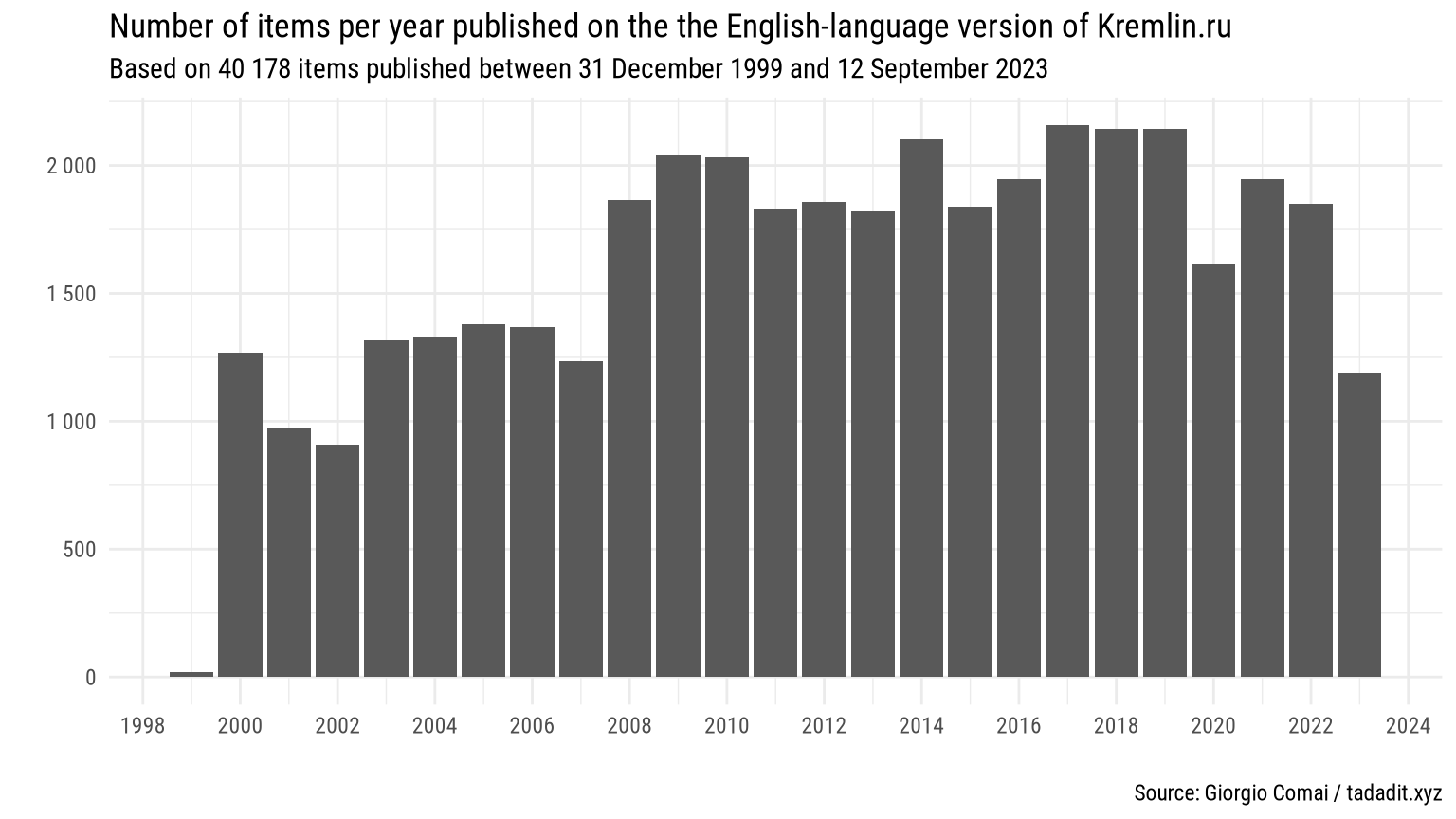
We see a slight increase in the number of posts since 2008, a slump in 2020 (covid-related?), but not much. Looking at the word count, we also see that the posts have been getting longer on average, so there’s more than three times as much text from recent years than on previous ones (which is relevant, as it impacts non-weighted word counts).
words_per_day_df <- corpus_df |>
  cas_count_total_words() |>
  mutate(date = lubridate::as_date(date),
         pattern = "total words")

words_per_day_df |>
  cas_summarise(period = "year", auto_convert = TRUE) |>
  rename(year = date) |>
    ggplot(mapping = aes(x = year, y = n)) +
  geom_col() +
  scale_y_continuous(name = "", labels = scales::number) +
  scale_x_continuous(name = "", breaks = scales::pretty_breaks(n = 10)) +
  labs(title = "Number of words per year published on the the English-language version of Kremlin.ru",
       subtitle = stringr::str_c("Based on ",
                                 scales::number(nrow(corpus_df)),
                                 " items published between ",
                                 format.Date(x = min(corpus_df$date), "%d %B %Y"),
                                 " and ",
                                 format.Date(x = max(corpus_df$date), "%d %B %Y")),
       caption = "Source: Giorgio Comai / tadadit.xyz")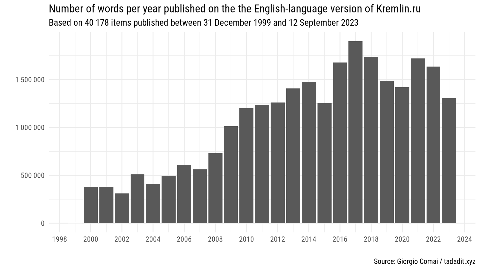
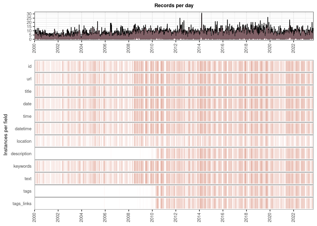
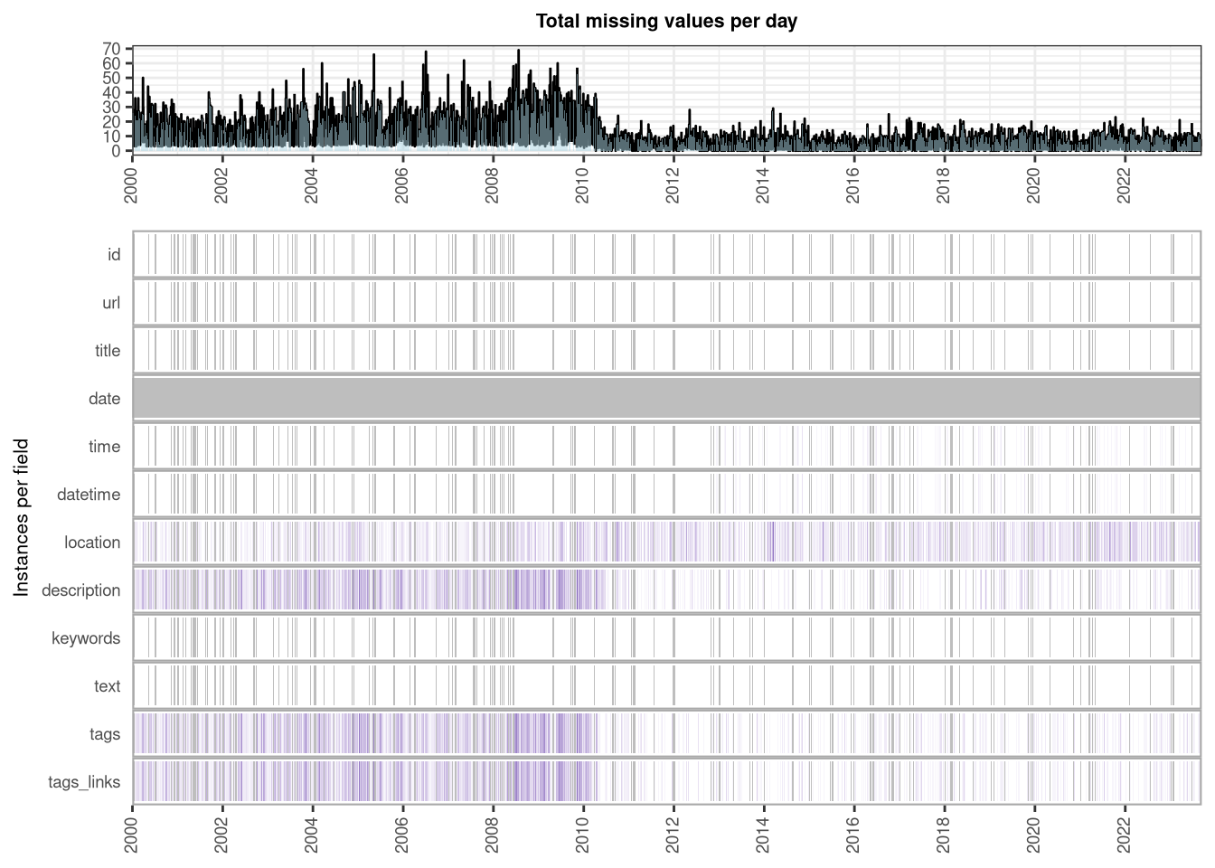
But these are just basic impressions about what is going on… in generale, it’s a good idea to make some proper data quality checks. A fully formalised approach to this part of the process will be detailed in a separate post, but we can achieve a lot of information on the availability of data by looking at the reports generated with the daiquiri package Quan (2022).
As the following graphs show, tags and description are available only starting with 2010. Location is often missing, but it is occasionally available starting with the early years. Depending on the type of analysis we are interested in, these data may need to go through some further quality checks, but at its most basic, things look as expected.
Step 10: Archive and backup
All looks good, and we can move on to create other textual datasets or to analyse what we have collected. But to keep things in good order, it’s a good idea to compress the tens of thousands of html files we have downloaded to free up some space.
This can be easily achieved with the following command.
cas_archive()You will find yourself with some big compressed files that can be stored in a backup on your favourite service. The local database keeps track of which file is where.
Depending on the type of dataset you are working on, it may make sense to ensure that you are not the only person to hold a copy of the original source. The following functions check if the original pages exist on the Internet Archive Wayback Machine, and if they are not, they try, very slowly, to add them to the archive. All of the Kremlin’s website is available there already, so no issues in this case, but for smaller websites I feel there is some use in ensuring their long term availability. More efficient approaches to achieve the same result will be considered.
cas_ia_check()

cas_ia_save()
Step 11: Keep the dataset updated
This is quite easy, as this is part of the whole point of having built castarter, but I will describe this in a separate post.
Step 12: At long last, look at the data
Here’s just a couple of quick examples for reference. But here is where this tutorial ends, and the actual content analysis begins.
corpus_df |>
  cas_count(pattern = "Ukrain") |>
  cas_summarise(period = "year",
                auto_convert = TRUE) |>
  rename(year = date) |>
    ggplot(mapping = aes(x = year, y = n)) +
  geom_col() +
  scale_y_continuous(name = "", labels = scales::number) +
  scale_x_continuous(name = "", breaks = scales::pretty_breaks(n = 10)) +
  labs(title = stringr::str_c("Number of mentions of ",
                              sQuote("Ukraine"),
                              " per year on Kremlin.ru"),
       subtitle = stringr::str_c("Based on ",
                                 scales::number(nrow(corpus_df)),
                                 " items published in English between ",
                                 format.Date(x = min(corpus_df$date), "%d %B %Y"),
                                 " and ",
                                 format.Date(x = max(corpus_df$date), "%d %B %Y")),
       caption = "Source: Giorgio Comai / tadadit.xyz")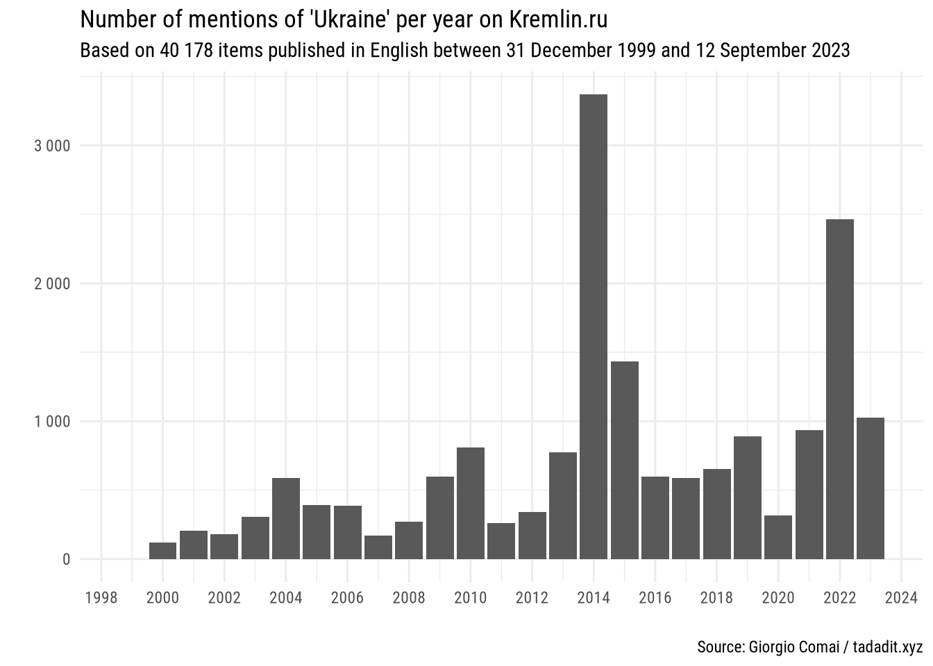
corpus_df |>
  cas_count(pattern = "Collective West") |>
  cas_summarise(period = "year",
                auto_convert = TRUE) |>
  rename(year = date) |>
    ggplot(mapping = aes(x = year, y = n)) +
  geom_col() +
  scale_y_continuous(name = "", labels = scales::number) +
  scale_x_continuous(name = "", breaks = scales::pretty_breaks(n = 10)) +
  labs(title = stringr::str_c("Number of mentions of ",
                              sQuote("Collective West"),
                              " per year on Kremlin.ru"),
       subtitle = stringr::str_c("Based on ",
                                 scales::number(nrow(corpus_df)),
                                 " items published in English between ",
                                 format.Date(x = min(corpus_df$date), "%d %B %Y"),
                                 " and ",
                                 format.Date(x = max(corpus_df$date), "%d %B %Y")),
       caption = "Source: Giorgio Comai / tadadit.xyz")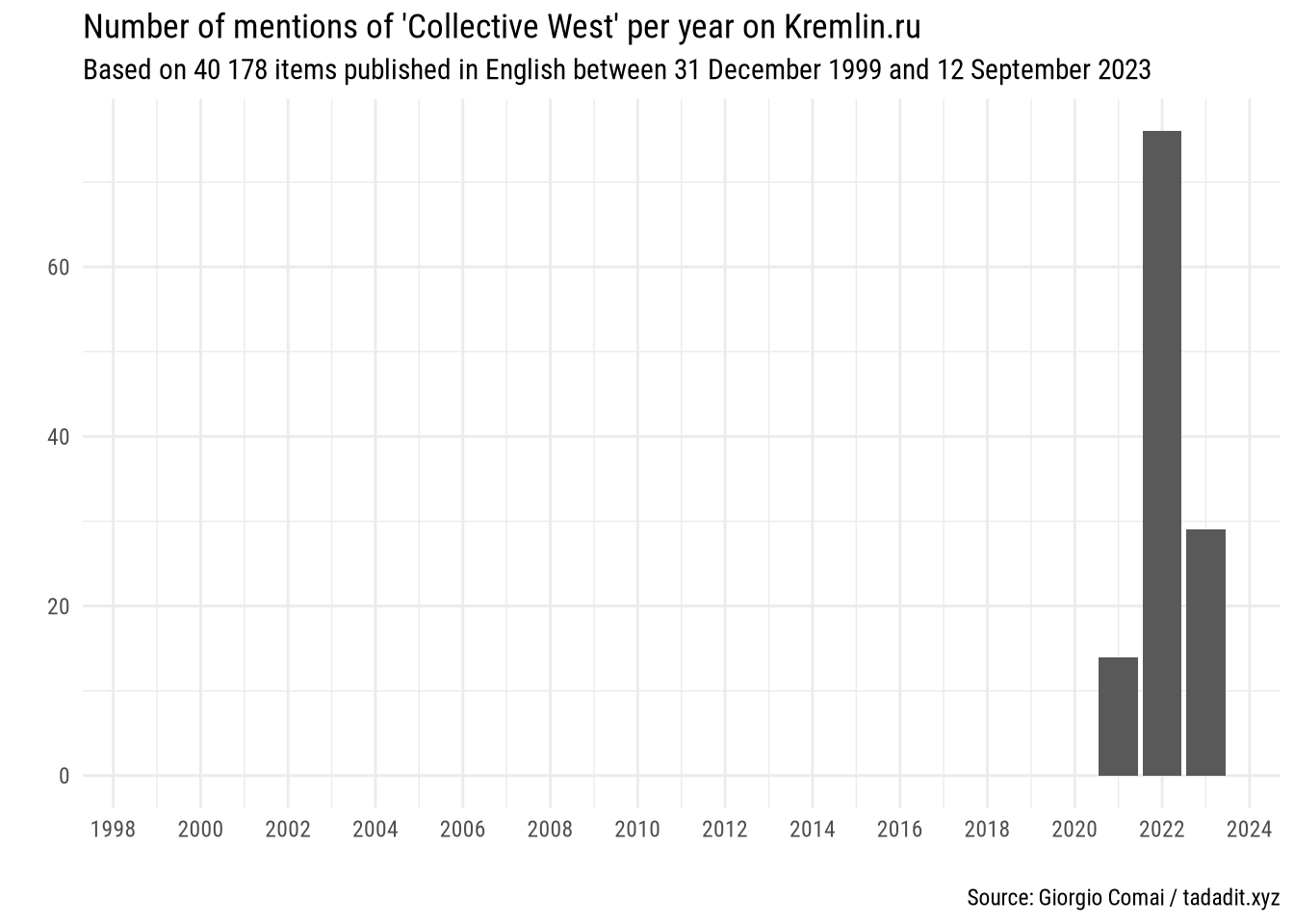
For an example of basic content analysis on a dataset such as this one, see the post: “Who said it first? ‘The collective West’ in Russia’s nationalist media and official statements”
References
Quan, T. Phuong. 2022. “Daiquiri: Data Quality Reporting for Temporal Datasets.” Journal of Open Source Software 7 (80): 5034. https://doi.org/10.21105/joss.05034.